
Exponential functions are mathematical expressions of the form y = ab^x‚ where ‘b’ is the base and ‘a’ is a coefficient. They are fundamental in mathematics and science‚ describing growth or decay patterns. Understanding these functions is essential for modeling real-world phenomena‚ such as population growth or radioactive decay. This section provides a comprehensive overview of exponential functions‚ their properties‚ and their applications‚ serving as a foundation for further study.
1.1 Definition and Basic Form
An exponential function is a mathematical expression of the form y = ab^x‚ where ‘a’ is a coefficient‚ ‘b’ is the base‚ and ‘x’ is the exponent. The base ‘b’ must be positive and not equal to 1‚ while ‘a’ can be any real number. Exponential functions are classified into two categories: growth (b > 1) and decay (0 < b < 1). The basic form y = ab^x serves as the foundation for understanding more complex exponential expressions. This fundamental structure is essential for graphing and analyzing exponential behavior‚ as it determines key features like asymptotes and intercepts.
1.2 Importance of Graphing Exponential Functions
Graphing exponential functions is crucial for visualizing their behavior and understanding their real-world applications. By plotting functions like y = ab^x‚ one can identify growth or decay patterns‚ asymptotes‚ and intercepts. This visual representation aids in predicting future trends‚ such as population growth or radioactive decay. Graphing also helps in comparing different exponential functions‚ highlighting similarities and differences. Additionally‚ it provides a practical way to verify solutions to equations and model complex phenomena. Regular practice through worksheets ensures proficiency in interpreting and sketching exponential graphs‚ a skill vital for advanced mathematics and science courses.

Characteristics of Exponential Function Graphs
Exponential function graphs exhibit distinct shapes‚ often curving upward or downward. They possess horizontal asymptotes‚ influencing end behavior‚ and can demonstrate either exponential growth or decay‚ depending on the base.
2.1 Asymptotes and End Behavior
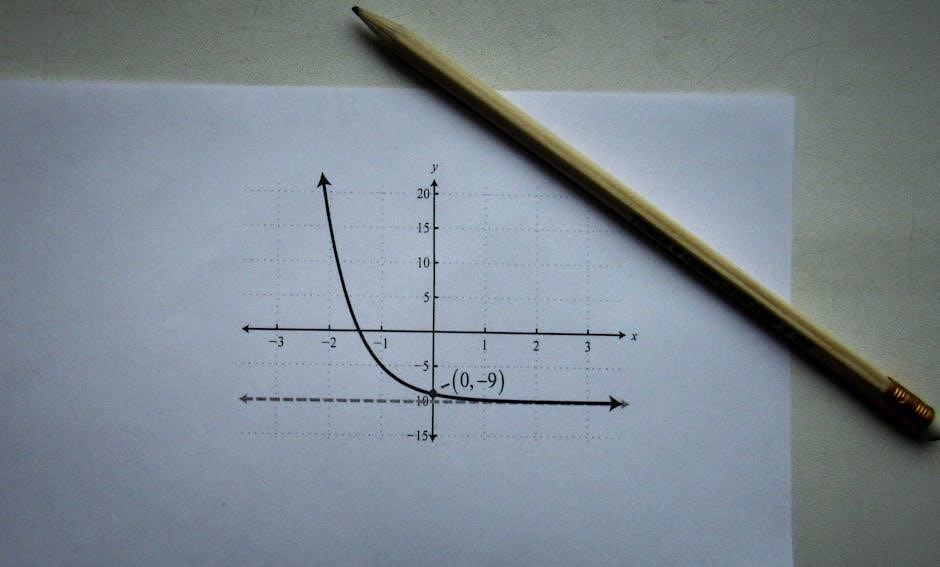
Exponential functions often have horizontal asymptotes‚ typically y = 0‚ which the graph approaches but never touches. For y = ab^x‚ if b > 1‚ the function grows rapidly as x increases and approaches the asymptote as x decreases. If 0 < b < 1‚ the behavior reverses: the function decays toward the asymptote as x increases. End behavior is crucial for sketching graphs‚ as it determines how the curve aligns with its asymptote and whether it rises or falls. Understanding these characteristics helps in accurately graphing exponential functions and interpreting their growth or decay patterns.
2.2 Identifying Growth and Decay
Exponential functions exhibit either growth or decay based on their base. For y = ab^x‚ if b > 1‚ the function shows exponential growth‚ increasing rapidly as x rises. If 0 < b < 1‚ the function demonstrates exponential decay‚ decreasing as x increases. Growth is identified by an upward curve‚ while decay results in a downward curve. These behaviors are crucial for interpreting real-world applications‚ such as population growth or radioactive decay. By analyzing the base‚ one can determine whether the function models growth or decay‚ aiding in accurate graphing and data interpretation.
2.3 Key Features: Domain‚ Range‚ and Intercept
Exponential functions have distinct characteristics that define their behavior. The domain of an exponential function y = ab^x is all real numbers‚ as exponential functions are defined for any x-value. The range‚ however‚ depends on whether the function exhibits growth or decay. For growth functions (b > 1)‚ the range is (a‚ ∞)‚ while for decay functions (0 < b < 1)‚ the range is (0‚ a). The y-intercept occurs at x = 0‚ giving the point (0‚ a). Understanding these features is essential for accurately graphing and interpreting exponential functions in various mathematical and real-world contexts.

Graphing Exponential Functions: Step-by-Step Guide
Start by identifying the function type and key features. Plot points to outline the curve‚ locate the y-intercept‚ and determine the horizontal asymptote. Sketch the graph‚ distinguishing between growth and decay based on the base value‚ ensuring accuracy and clarity in your visualization.
3.1 Plotting Points and Drawing the Curve
To graph an exponential function‚ begin by identifying the function and its form. Create a table of x and y values to plot key points. Identify the y-intercept and horizontal asymptote to guide your sketch. For growth functions (b > 1)‚ the curve rises rapidly; for decay functions (0 < b < 1)‚ it decreases gradually. Plot points accurately‚ ensuring the curve approaches the asymptote. Use smooth lines to connect points‚ reflecting the function's behavior. This method ensures clarity and precision in visualizing exponential growth or decay patterns for analysis and interpretation.
3.2 Using a Graphing Calculator
Utilize a graphing calculator to efficiently plot exponential functions. Enter the function in the calculator’s equation editor‚ ensuring correct syntax. Adjust the window settings to display the function’s key features‚ such as asymptotes and intercepts. Use zoom and trace functions to analyze behavior at specific points. Identify growth or decay patterns visually and verify with calculations. This tool simplifies graphing‚ especially for complex functions‚ and allows for quick adjustments to explore transformations or compare multiple functions side by side. Regular practice with a graphing calculator enhances understanding and accuracy in graphing exponential functions.
3.3 Transformations: Horizontal and Vertical Shifts
Exponential functions can undergo horizontal and vertical shifts‚ altering their graphs without changing their basic shape; Vertical shifts occur when a constant is added to the function‚ such as y = ab^x + c‚ moving the graph up or down. Horizontal shifts involve adding a constant inside the exponent‚ like y = ab^(x ⎼ h)‚ shifting the graph left or right. These transformations are crucial for modeling real-world phenomena and analyzing function behavior. Practice worksheets often include identifying and graphing these shifts‚ reinforcing understanding of how they affect the function’s key features and overall appearance on a coordinate plane.

Common Types of Exponential Functions
Exponential functions are categorized into natural (base e)‚ binary (base 2)‚ and decimal (base 10) types‚ each with distinct applications in graphing and real-world analysis.
4.1 Natural Exponential Functions (Base e)
Natural exponential functions are of the form y = e^x‚ where e is approximately 2.71828. These functions are crucial in calculus and real-world applications‚ such as finance and biology. The function e^x grows rapidly as x increases and approaches zero as x decreases. It has a horizontal asymptote at y = 0 and passes through (0‚1). Natural exponentials are used to model continuous growth rates‚ such as compound interest‚ and are essential for understanding derivatives and integrals. Graphing these functions helps visualize their behavior and solve practical problems‚ making them a cornerstone of mathematical analysis.
4.2 Binary Exponential Functions (Base 2)
Binary exponential functions are of the form y = 2^x‚ where the base is 2. These functions are fundamental in computer science and digital technology‚ as they model binary systems and growth in fields like algorithm complexity. The function y = 2^x grows exponentially as x increases and approaches zero as x decreases. Key points include (0‚1) and (1‚2)‚ illustrating rapid growth. These functions are widely used to describe population growth‚ compound interest‚ and technological advancements. Graphing y = 2^x helps visualize its exponential behavior‚ making it essential for understanding binary systems and their applications in modern computing and data analysis.
4.3 Decimal Exponential Functions (Base 10)
Decimal exponential functions‚ of the form y = 10^x‚ are widely used in scientific and real-world applications. The base 10 is common in measurements like pH levels‚ the Richter scale‚ and financial contexts such as investments and inflation. These functions grow rapidly as x increases and approach zero as x decreases. Key points include (0‚1) and (1‚10)‚ demonstrating exponential growth patterns. Graphing y = 10^x helps visualize its behavior‚ making it essential for understanding logarithmic relationships and scaling in various fields. This function is fundamental for modeling phenomena where base 10 is naturally occurring or required for simplicity and clarity.

Identifying Features from the Equation
Exponential functions’ equations reveal key features like bases‚ coefficients‚ and asymptotes. Analyzing these elements helps determine growth or decay patterns‚ intercepts‚ and end behavior‚ aiding accurate graphing and interpretation.
5.1 Coefficients and Bases
In exponential functions of the form y = ab^x‚ ‘a’ is the coefficient and ‘b’ is the base. The base ‘b’ determines the growth rate: if b > 1‚ the function grows exponentially‚ while if 0 < b < 1‚ it decays. The coefficient 'a' scales the function vertically‚ affecting the y-intercept. For example‚ in y = 2*3^x‚ 'a' is 2 and 'b' is 3‚ leading to rapid growth. Changing 'a' or 'b' alters the graph's shape and behavior‚ essential for modeling real-world scenarios like finance or biology.

5.2 Vertical and Horizontal Asymptotes
Exponential functions often have vertical asymptotes‚ which are horizontal lines the graph approaches but never touches. For y = ab^x‚ the vertical asymptote is typically y = 0‚ as the function approaches the x-axis as x approaches negative infinity. Horizontal asymptotes‚ which are vertical lines‚ do not exist for standard exponential functions since they grow without bound. Understanding asymptotes is crucial for sketching and analyzing the behavior of exponential functions‚ helping to identify limits and end behavior. They provide key insights into how the function behaves as x increases or decreases.
5.3 Determining Growth vs. Decay
Exponential functions either exhibit growth or decay based on the base ‘b.’ If b > 1‚ the function grows rapidly as x increases‚ with the graph rising steeply. Conversely‚ if 0 < b < 1‚ the function decays‚ approaching zero as x increases. To identify growth or decay‚ analyze the base: a larger base indicates faster growth‚ while a base between 0 and 1 signifies decay. This distinction is crucial for interpreting real-world applications‚ such as modeling population growth or radioactive decay‚ where understanding whether a quantity increases or decreases exponentially is essential for accurate predictions and analysis.
Practice Worksheet with Answers
This worksheet provides sample problems and solutions for graphing exponential functions. Practice identifying growth or decay‚ asymptotes‚ and key features while verifying answers for accuracy and understanding.
6.1 Sample Problems and Solutions
This section offers a variety of sample problems‚ each accompanied by detailed solutions. Problems range from graphing basic exponential functions to identifying asymptotes and determining growth or decay. Solutions include step-by-step explanations‚ ensuring clarity and understanding. For example‚ one problem asks to graph y = 2^x and identify its asymptote. The solution demonstrates plotting points like (0‚1) and (1‚2)‚ explaining the horizontal asymptote at y=0. Another problem involves determining if y = 3^{-x} shows growth or decay‚ with the solution explaining the decay behavior as the base is between 0 and 1. These exercises help solidify concepts through practical application.
6.2 Checking Work Using Asymptotes
Asymptotes are crucial for verifying the accuracy of exponential function graphs. For any function of the form y = ab^x‚ the horizontal asymptote can be identified by examining the behavior as x approaches infinity or negative infinity. For example‚ if the base b is greater than 1‚ the asymptote is y=0. If 0 < b < 1‚ the asymptote remains y=0. To check your work‚ compare the asymptote you've graphed with the expected one based on the equation. This step ensures your graph aligns with the function's mathematical properties and helps catch errors in plotting points or interpreting growth/decay patterns.
6.3 Common Mistakes and Corrections
When graphing exponential functions‚ common mistakes include misidentifying the base and coefficient‚ leading to incorrect growth or decay trends. For example‚ confusing a negative coefficient with the base can result in an inverted graph. Another error is miscalculating intercepts‚ such as the y-intercept‚ which occurs at x=0. To correct these‚ ensure the base is greater than 0 and not equal to 1‚ and accurately plot points by substituting x-values. Additionally‚ mislabeling asymptotes can occur; always confirm the horizontal asymptote aligns with y=0 for positive bases. Attention to detail and methodical plotting help avoid these pitfalls and ensure accurate graphs.

Real-World Applications
Exponential functions model population growth‚ radioactive decay‚ and financial growth. They are essential for predicting trends in these real-world fields.
7.1 Population Growth Models

Exponential functions are widely used to model population growth‚ where the rate of growth is proportional to the current population. The classic equation is ( P(t) = P_0 e^{rt} )‚ where ( P_0 ) is the initial population‚ ( r ) is the growth rate‚ and ( t ) is time. This model assumes unlimited resources‚ leading to rapid growth. However‚ real-world scenarios often incorporate limitations‚ transitioning to logistic growth models. Graphing these functions helps visualize how populations expand over time‚ making them essential tools in ecology and environmental science for predicting future trends and managing resources effectively.
7.2 Radioactive Decay
Exponential functions are crucial in modeling radioactive decay‚ where the amount of a substance decreases at a rate proportional to its current quantity. The decay process follows the formula ( N(t) = N_0 e^{-kt} )‚ where ( N(t) ) is the remaining quantity‚ ( N_0 ) is the initial amount‚ ( k ) is the decay constant‚ and ( t ) is time. Graphing these functions reveals a decreasing curve approaching zero asymptotically. This application is vital in nuclear physics‚ medicine‚ and environmental science‚ as it helps predict half-lives and understand the stability of radioactive materials. Accurate graphing aids in analyzing decay rates and their practical implications.

7.3 Financial Growth and Compound Interest
Exponential functions are essential in modeling financial growth‚ particularly in compound interest calculations. The formula ( A = P(1 + rac{r}{n})^{nt} ) illustrates how investments grow over time‚ where ( A ) is the amount‚ ( P ) is the principal‚ ( r ) is the interest rate‚ ( n ) is the number of times interest is compounded‚ and ( t ) is time. Graphing these functions reveals rapid growth over time‚ demonstrating the power of compounding; This application is vital for understanding investment strategies‚ retirement planning‚ and the long-term benefits of saving. Accurate graphing helps individuals make informed financial decisions and predict future wealth accumulation.
Mastering exponential functions is crucial for understanding growth and decay patterns. Practice with worksheets and real-world applications ensures proficiency in graphing and interpreting these essential mathematical concepts.
8.1 Summary of Key Concepts
Exponential functions‚ of the form y = ab^x‚ describe growth or decay patterns. Key concepts include identifying bases‚ coefficients‚ asymptotes‚ and determining domains and ranges. Understanding end behavior‚ intercepts‚ and transformations is crucial. Practice worksheets and real-world applications‚ such as population growth and financial calculations‚ reinforce these principles. Mastering graphing techniques and interpreting function characteristics ensures proficiency in analyzing exponential relationships. Regular practice and reviewing common mistakes aid in solidifying these fundamental mathematical skills‚ essential for advanced problem-solving across various disciplines.
8.2 Importance of Practice
Consistent practice is crucial for mastering the graphing of exponential functions. It reinforces understanding of key concepts such as asymptotes‚ growth vs. decay‚ and transformations. Worksheets with answers provide opportunities to check work‚ identify mistakes‚ and improve accuracy. Regular practice helps develop problem-solving skills and builds confidence in analyzing exponential relationships. Additionally‚ it prepares students for real-world applications‚ such as population modeling and financial calculations‚ where precise graphing is essential. By dedicating time to practice‚ learners can solidify their knowledge and achieve proficiency in this fundamental area of mathematics.
8.3 Resources for Further Study
For deeper understanding‚ numerous resources are available‚ including worksheets with answers‚ online tutorials‚ and graphing calculators. Kuta Software’s Infinite Algebra 2 offers comprehensive practice materials. Websites like Khan Academy and Mathway provide step-by-step guides and interactive tools. Additionally‚ textbooks and educational platforms often include detailed sections on exponential functions. Utilizing these resources can enhance learning and reinforce concepts such as asymptotes‚ transformations‚ and real-world applications. They also offer varied problem sets to ensure mastery of graphing exponential functions‚ making them invaluable for students seeking additional support or challenging exercises.